Seccions verticals de gràfics de funcions de dues variables

Secció vertical en \(x=\)constant

JA hem vist com fer aquesta mena de gràfiques:

library(rgl)
# primer definim la funció
f <- function(x,y) return(x^2 - y^2)

# definim els valors de x i de y on volem avaluar la funció
X <- seq(-1, 1, length = 10)
Y <- seq(-1, 1, length = 10)
# i ara fabriquem una matriu de valors z per cada parella x, y  
Z <- outer(X,Y,f)

# ja podem graficar:
surface3d(X,Y,Z, col="orange", back="lines", alpha=0.5, lit=FALSE)
axes3d(edges=c("x-", "y-", "z-"))
title3d(xlab="x", ylab="y", zlab="z")

Ara hi afegin una línia blava per valors constants de \(x=0.5\).

ct = 0.5
zli = f(ct, Y)
lines3d(x=rep(ct,length=10), y=Y, z=zli, lwd=3, alpha=0.5, col="blue")

I una línia vermella per valors constants de \(y=0.5\)

ct = 0.5
zli = f(X,ct)
lines3d(x=X, y=rep(ct,length=10),z=zli, col="red", lwd=3, alpha=0.5)

Hauries d’obtenir alguna cosa com això, i ho podras girar per entendre millor el que es veu. La linia blava correspon a valors fixos de \(x=0.5\) amb \(z=z(y)=f(0.5,y)=0.25-y^2\), és per tant una paràbola amb les banyes avall. La linia vermella correspon a valors fixos de \(y=0.5\) amb \(z=z(x)=f(x, 0.5)=x^2-0.25\), és per tant una paràbola amb les banyes amunt.

An advanced script (M. Greenacre)

This script is not evaluated here, you may copy and paste it to the RStudio script window and execute it step by step.

### Script to graph 2-variables functions, with vertical cuts and animation
### courtesy of Michael Greenacre, december 2020

### Execute the parts between ### ------ one part at a time

### -------------------------------------------------------------------------
### non linear function with two intersecting planes

### The following changes depending on the function, which I call mates2
### Define the function to be plotted...
mates2 <- function(x,y) {
  result <- NA
  z <- x^2 / y           ### change this line for different function                              
  if(is.finite(z)) result <- z
  result
}

### -------------------------------------------------------------------------
### ...and the limits of the (x,y) values for plotting:
xlim<-c(-1,1)                                      
ylim<-c(0.5,3) 

require(rgl)

### define function on a 51x51 domain grid (steps of 1/50th)
points<-51
x<-seq(xlim[1],xlim[2],(xlim[2]-xlim[1])/(points-1))
y<-seq(ylim[1],ylim[2],(ylim[2]-ylim[1])/(points-1))

### values of function on the grid
z<-matrix(0, nrow=points, ncol=points)
for(j in 1:points){
  for(i in 1:points){
  z[i,j] <- mates2(x[i],y[j])
  }
}
ztemp <- as.numeric(z)
zlim  <- range(na.omit(ztemp))
zmin  <- zlim[1]
zmax  <- zlim[2]
ztemp <-as.numeric(z)
zlim  <- range(na.omit(ztemp))
zlen  <- zlim[2]-zlim[1]

### height colour lookup table
colorlut <- terrain.colors(zlen) 
### assign colours to heights for each point
col   <- colorlut[na.omit(z)-zlim[1]+1 ]

### 3D plotting
# open3d()  
clear3d()
view3d(theta = 20, phi = 10 , fov = 20, zoom=0.9) 
rgl.surface(x, y, z, color="forestgreen", back="lines", asp=1)

### draw axes (Note: here x is first axis, z the second and y the third)
### This means that "y" comes "out" and "z" and "x" are the facing "wall"
lines3d(c(0,1.05*xlim[2]), c(0,0), c(0,0), col="blue", lty=2)
lines3d(c(0,0), c(0,0), c(0,1.05*ylim[2]), col="blue")
lines3d(c(0,0), c(1.05*zmin,1.05*zmax), c(0,0),col="blue")

### axis labels
text3d(1.15*xlim[2], 0, 0, "x", font=4, cex=1.3, col="blue")
text3d(0, 1.1*zmax, 0, "z", font=4, cex=1.3, col="blue")
text3d(0, 0, 1.1*ylim[2], "y", font=4, cex=1.3, col="blue")

### add upper limits of axes
text3d(0, -.03, ylim[2], ylim[2], font=2, col="blue")
text3d(xlim[2], -0.1, 0, xlim[2], font=2, col="blue")
text3d(-0.1, zmax, -0.1, zmax, font=2, col="blue")
text3d(-0.1, zmin, -0.1, zmin, font=2, col="blue")

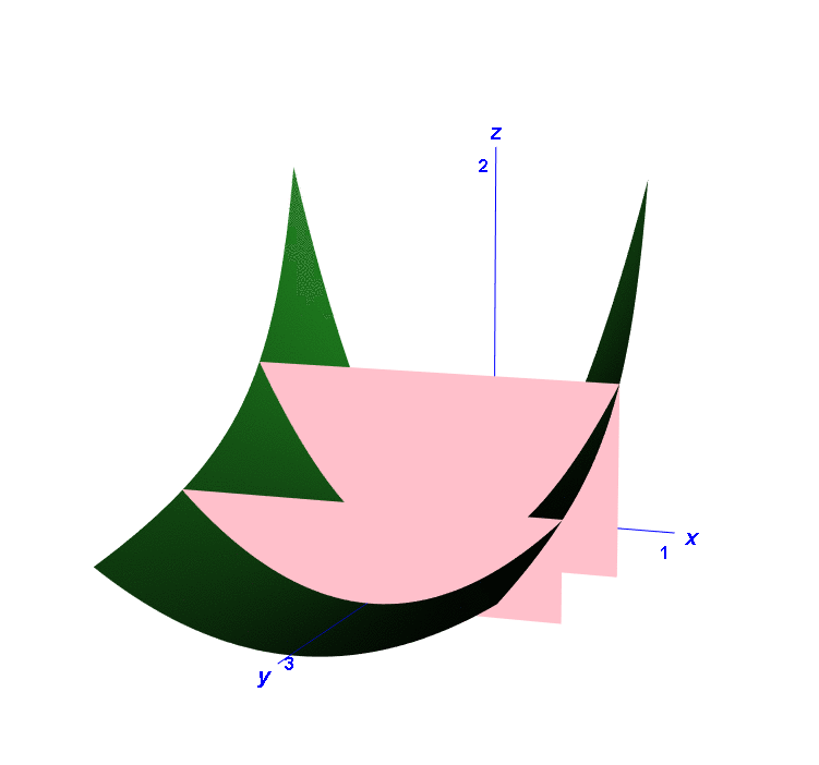
### the cutting plane at y=2
### (custom-built plot "by hand" as a series of lines)
ycut <- 2
zcut <- mates2(xlim[2], ycut)
for(k in 0:100) {
  lines3d(c(xlim[1],xlim[2]), c(zcut*(k-1)/100,zcut*(k-1)/100), c(ycut,ycut), col="pink", lwd=3)
}
### the cutting plane at y=1
ycut <- 1
zcut <- mates2(xlim[2], ycut)
for(k in 0:100) {
  lines3d(c(xlim[1],xlim[2]), c(zcut*(k-1)/100,zcut*(k-1)/100), c(ycut,ycut), col="pink", lwd=3)
}

### now open that 3D graphics window to the required size, 
### and can zoom in or out with the mouse wheel
### (I opened to approx. 6 x 6 inches and then zoomed in slightly)

### -----------------------------------------------------------------------------

### now two choices:
### 1. To save the movie frames rotating about the z-axis in your working directory
movie3d(spin3d(c(0,1,0)), duration = 12, convert=FALSE, frames="nonlinear_two_cuts", dir=getwd())
### then I use an external program (in my case Animation Shop) to compile the frames to a video

### 2. But in latest versions of R there is an interface with magick package to create the movie in R
require(magick)
### The following takes a minute or two to make the GIF movie
movie3d(spin3d(c(0,1,0)), duration = 12, movie="nonlinear_movie", frames="nonlinear_two_cuts", dir=getwd())

You may obtain things like this. Even animated!

Seccions verticals de gràfics de funcions de dues variables

f.u. et al.

Obre Rstudio per seguir aquesta activitat

Secció vertical en \(x=\)constant

An advanced script (M. Greenacre)